James Tone Stack - Analysis
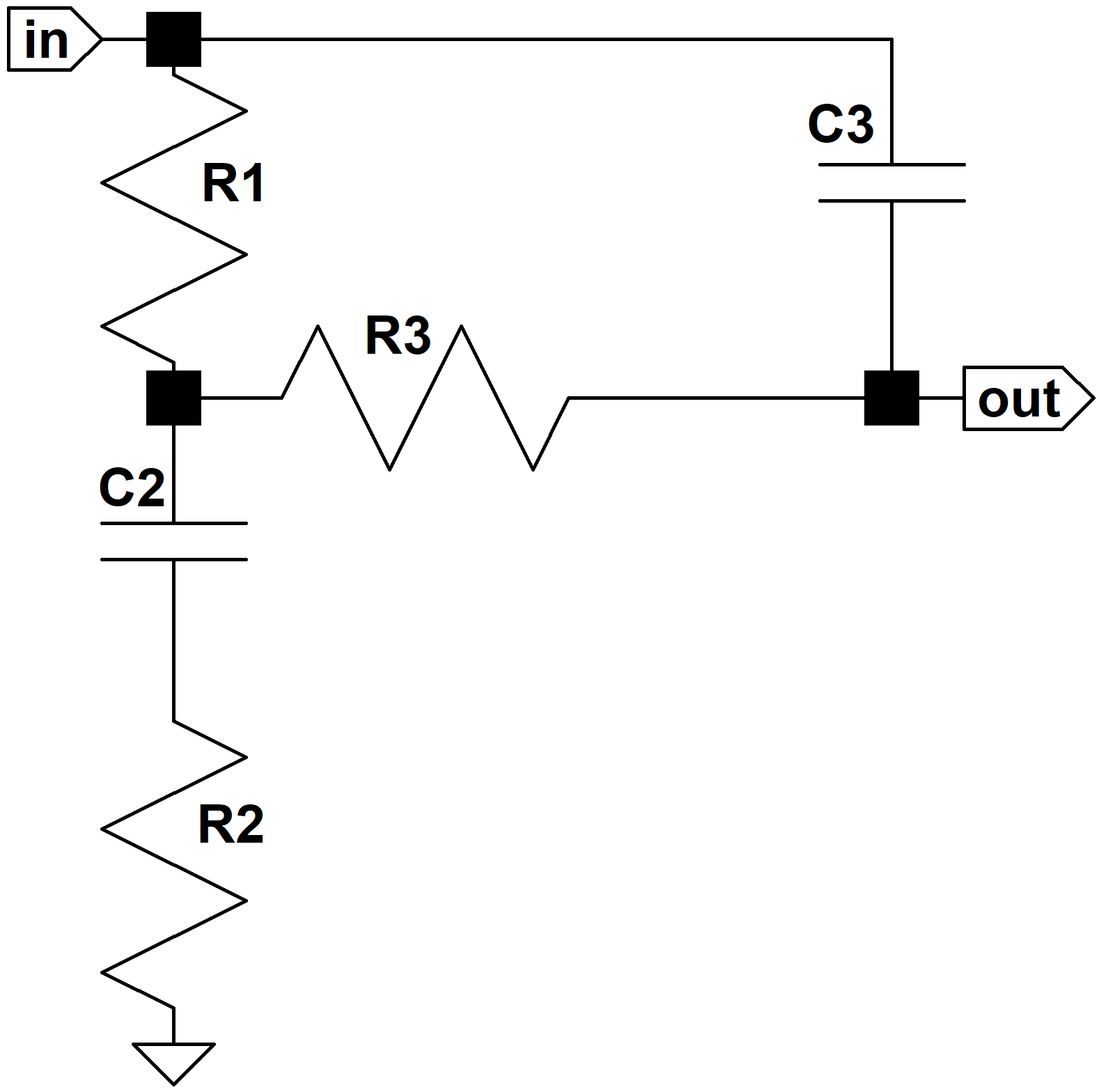
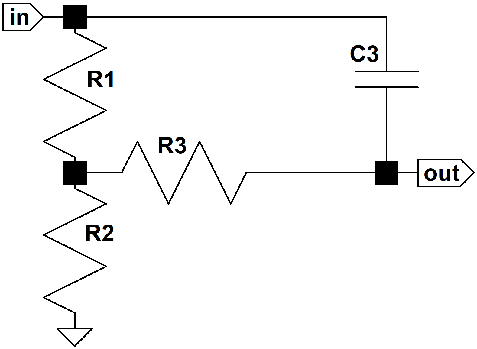
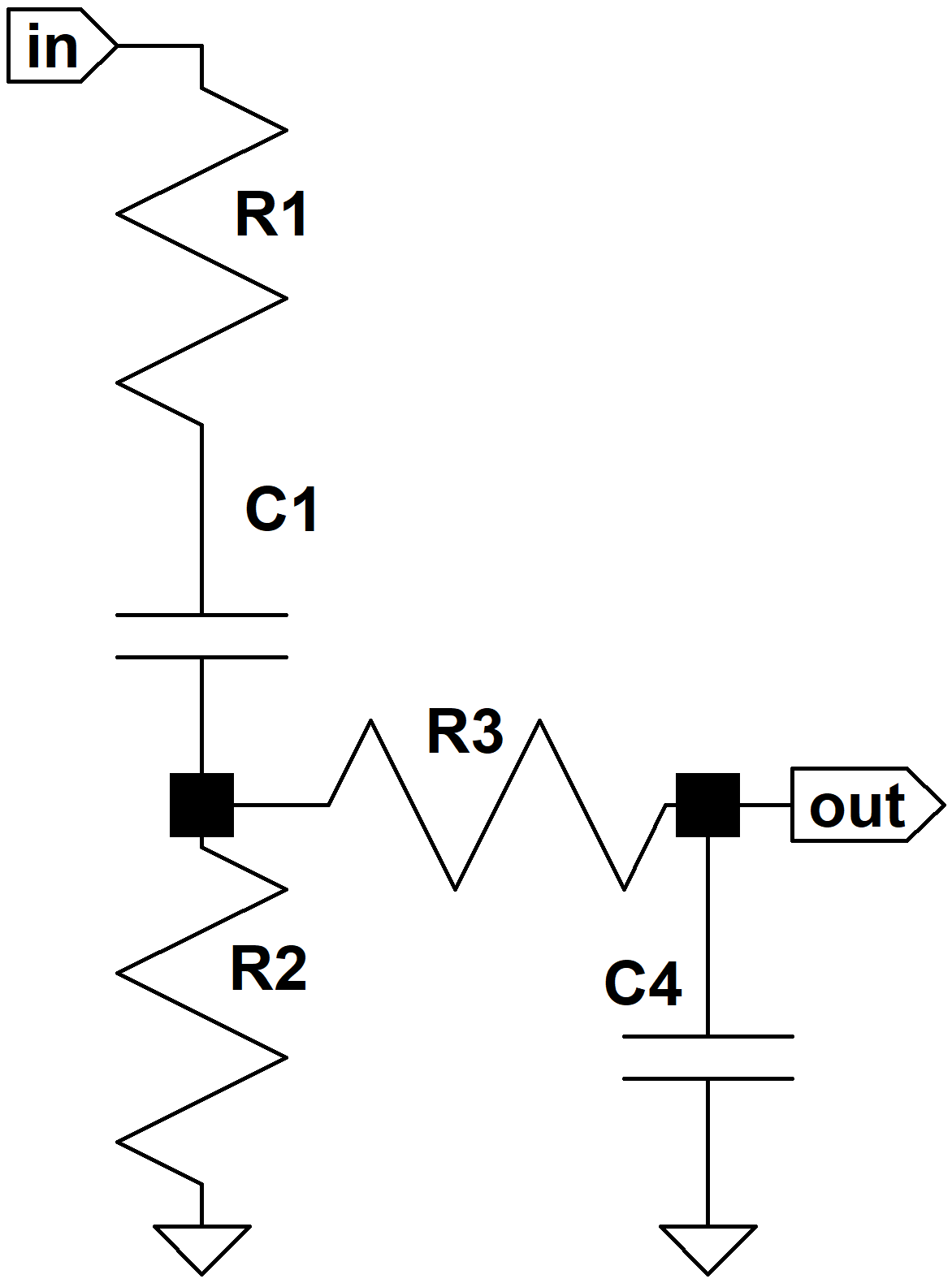
Here is the classic James Tone Stack as used, for example, in the 120-watt Orange Graphic.
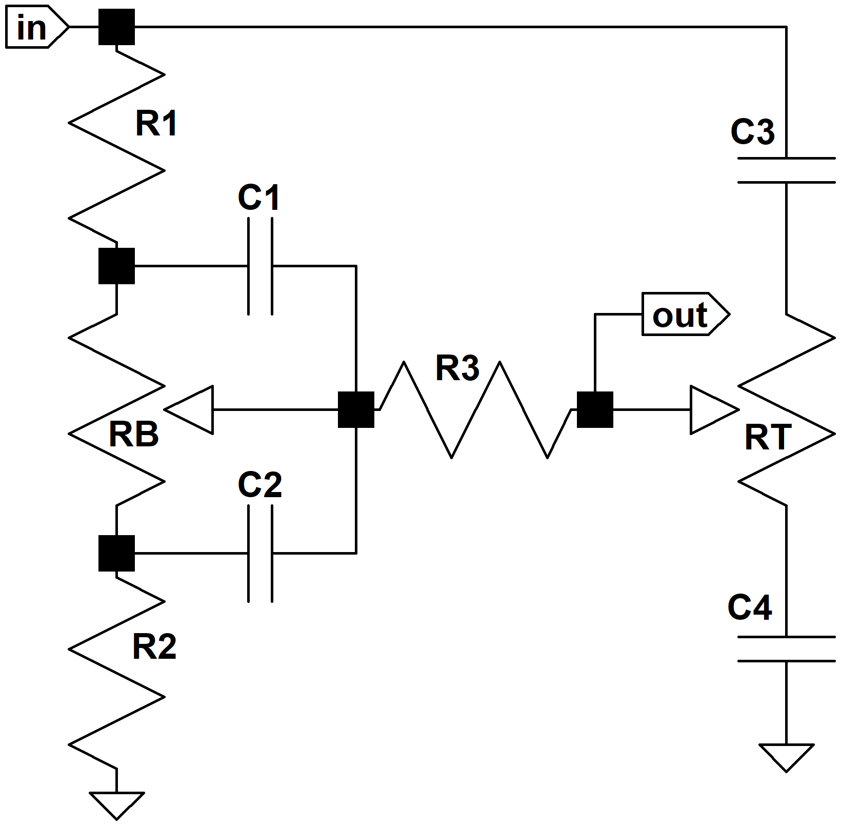
To keep the mathematics from becoming overwhelming, we'll make a few assumptions. First, we'll assume that the driving circuit has an output impedance of zero. For a low-impedance driver like a cathode follower, this is a highly-accurate assumption. A typical 12AX7 voltage amplifier, however, has an output impedance of almost 40kΩ, which reduces the accuracy of our formulas. Second, we'll assume tone control resistances are infinite, because typical 1MΩ controls have much greater resistance than the other impedances in the circuit. Finally, we'll assume that the tone stack output drives an infinite input impedance. Typically the input impedance to the next stage is at least 1MΩ.
These assumptions make it easier to design the James tone stack and calculate the required parts values. Once the circuit is finalized we can test the results under real circuit conditions.
|
Guitar Amplifier Electronics: Fender Deluxe - from TV front to narrow panel to brownface to blackface Reverb |
Controls at Maximum
Let's begin by setting the bass and treble controls at maximum. This shorts C1 and connects R3 to C3. Because we're assuming the control potentiometers have much larger values than the fixed resistors, their resistances are effectively disconnected from the circuit.
Low Frequencies
C3 is smaller than C2 and dominates performance only at treble frequencies. At bass and midrange frequencies we'll assume it is an open circuit. This approximation will prove very helpful in understanding circuit performance. In the spirit of divide-and-conquer, we'll look only at the low frequencies first.
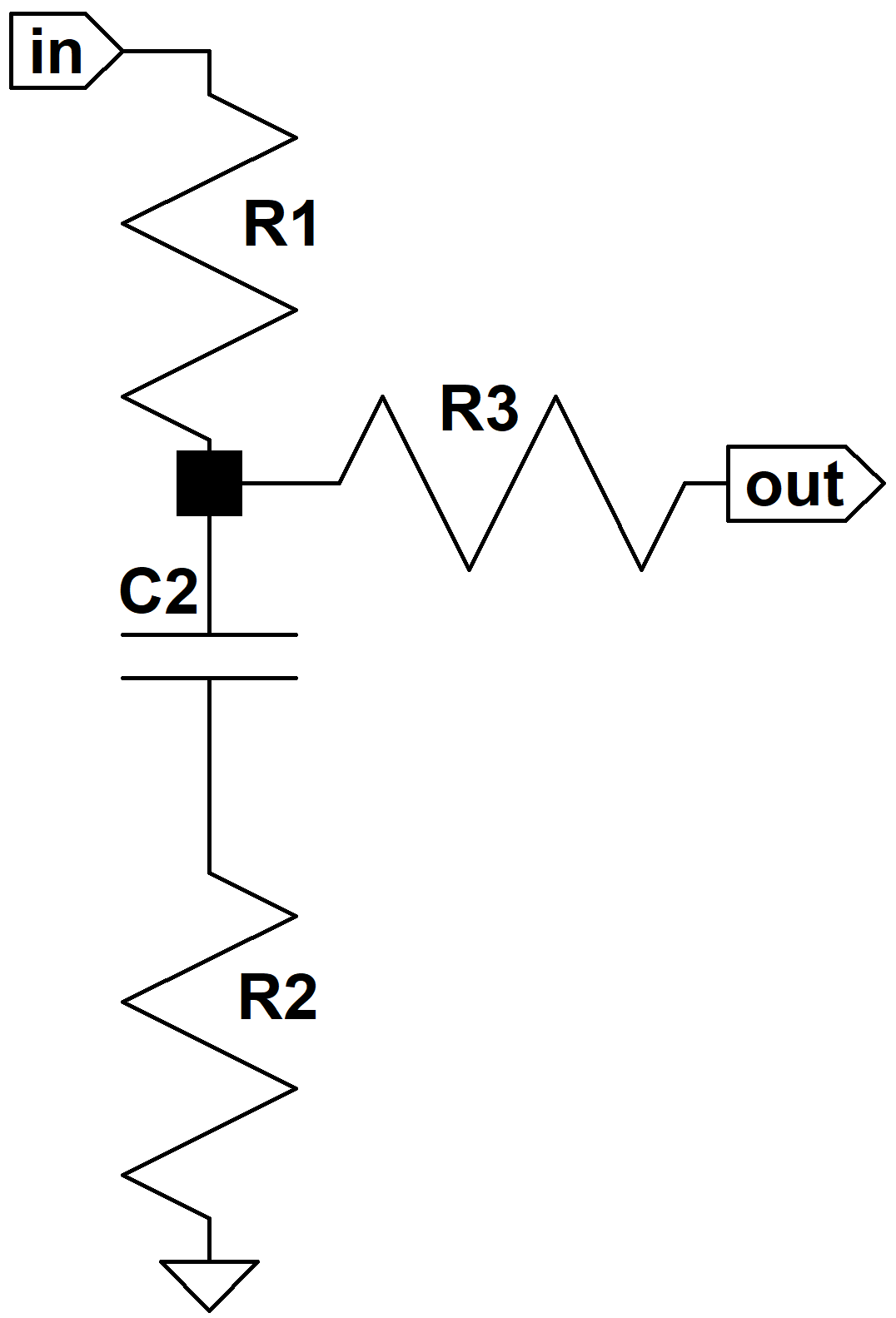
Because we're driving an open circuit, there is no current through R3 and by Ohm's Law there is no voltage across it. Thus we can treat it as a short circuit, giving us a classic voltage divider with a series impedance Z1 and shunt impedance Z2. In this case Z1 = R1 and Z2 is equal to the impedance of R2 in series with the capacitor impedance. The frequency response is then
(Our tutorials, lessons 8 to 11, explain complex impedance. If the variable "s" looks unfamiliar, please see our tutorial on Laplace notation.)
|
Guitar Amplifier Electronics: Basic Theory - master the basics of preamp, power amp, and power supply design. |
With some re-arranging we get the following formula suitable for creating a Bode magnitude plot:
where
There is a zero at s = -b and a pole at s = -a. Let's look at the extremes of frequency. At DC, where s = 0, we get H(s) = 1, so there is no attenuation. As the frequency goes to infinity we get
This makes sense, because at very high frequencies the capacitor is a short circuit and we get just a voltage divider formed by R1 and R2. This represents midrange attenuation. There is a transition frequency based on the pole:
Above this frequency the response transitions to its midrange value, decreasing at a rate of 6dB per octave (20dB per decade) until we reach the bass-midrange transition frequency based on the zero:
Here we are arriving at midrange, and the response is only 3dB above its final midrange value of
|
Fundamentals of Guitar Amplifier System Design - design your amp using a structured, professional methodology. |
Let's say all this once more and then introduce some hard numbers to make it even more clear. We have the bass control set to maximum, so we have no attenuation at very low frequencies. At the first transition frequency attenuation begins, ultimately decreasing at a rate of 20dB per decade until we reach the bass-midrange transition frequency where the gain levels off at a steady midrange attenuation value that lasts until we reach treble frequencies and C3 starts conducting significant current.
Now for some hard numbers.
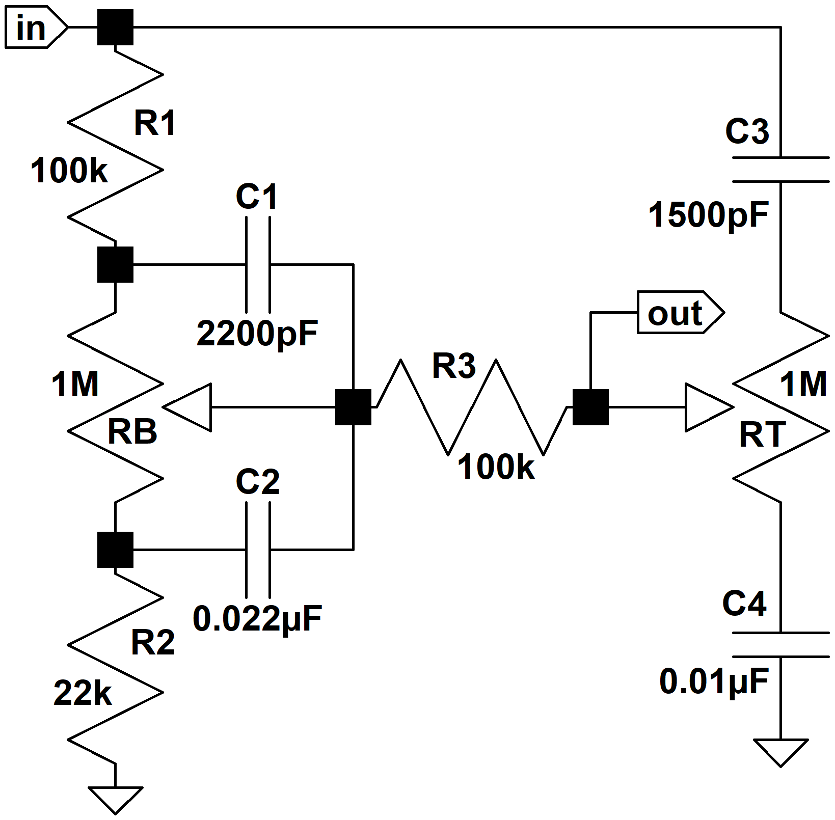
The Orange Graphic uses R1 = 100k, R2 = 22k, and C2 = 0.022uF. This means the midrange gain is -15dB. At low bass frequencies there is no attenuation. When the frequency rises to
which is 59 Hz, the gain has fallen by 3dB and is starting to decrease at a rate of 20dB per decade. It finally starts leveling off at the bass-midrange transition frequency of
which is 329Hz. At this point the gain is 3dB above its midrange value of -15dB.
|
Guitar Amplifier Electronics: Circuit Simulation - know your design works by measuring performance at every point in the amplifier. |
Now we are ready to draw the Bode magnitude plot for low and midrange frequencies with the bass control at maximum. For the pole we draw a horizontal line at 0dB until we reach the transition frequency of 59Hz. Then we draw a line sloping downward at the rate of 20dB per decade. For the zero we also draw a horizontal line at 0dB until we reach 329Hz, where we then draw a line sloping upward at 20dB per decade. The actual frequency response is very close to the sum of these two approximations. Here is the plot.
The approximate pole response and the approximate zero response are the dotted and dashed lines, respectively. The actual response, which includes the 3dB differences at the transition points, is the solid curve.
High Frequencies
At high frequencies C2 acts as a short circuit and C3 comes into play.
The frequency response is
This makes sense, because at DC, where s = 0, the response is
The capacitor is an open circuit at DC, there is no current through R3 and thus no voltage drop across it. Thus the output voltage is equal to the input voltage reduced in magnitude by the voltage divider formed by R1 and R2.
At extremely high frequencies, as s goes to infinity, the response becomes
This also makes sense, because at infinitely high frequencies the capacitor is a short circuit.
When R3 = R1, as in the Orange Graphic and many other designs, the response becomes
where
From these formulas we see that there is a gain of b/a and transition frequencies for a pole at -a and a zero at -b:
The second represents the midrange-treble transition frequency and the first represents a transition to zero attenuation at high treble frequencies. The gain thus begins at the midrange level created by the voltage divider formed by R1 and R2. It then breaks upward due to the zero at the midrange-treble transition frequency, ultimately rising at a maximum rate of 20dB per decade. Finally it breaks back to a flat response at the second transition frequency due to the pole.
The Orange Graphic uses C3 = 1500pF, for which the transition frequencies are 162Hz and 900Hz. Here is the Bode magnitude plot.
Here are the two Bode plots superimposed. The bass-to-midrange plot is only valid at low frequencies and the midrange-to-treble plot is only valid at high frequencies. The complete response is a gradual combining of the two plots.
Our calculations assume an ideal source, an ideal load, and infinite-impedance tone controls. Here is the actual response using Electronics Workbench Multisim®. The plot assumes 1MΩ tone controls, a driving circuit output impedance of 49k (using the Orange Graphic's 220k plate load resistor), and a driven circuit input impedance of 1MΩ.
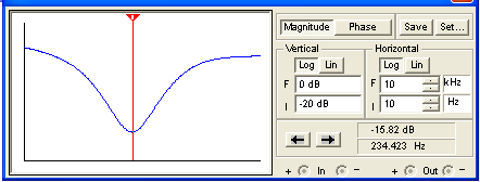
(The horizontal axis is a log scale of frequency from 10Hz to 10kHz and the vertical scale is from -20dB to 0dB.) We see that the real world impedances of the driving and driven circuits cause additional attenuation, but otherwise there are no surprises. Maximum attenuation occurs right where we expect.
Bass and Treble Controls at Minimum
When the tone controls are set to minimum we get this circuit:
which has this frequency response:

When R3 = R1 then this simplifies, at least slightly, to

For reasonable values, in particular when R1 and R3 are equal and substantially larger than R2, then the response is approximately
where
At DC, where s = 0, and at infinitely high frequencies, where s approaches infinity, the equation shows that the response is zero, which makes sense when the controls are at minimum because at DC the capacitor C1 is an open circuit and at the extremes of treble capacitor C4 is a short circuit.
There is a zero at s = 0 and there are poles at s = -a1 and s = -a2. The -3dB transition frequencies for the two poles are
At extremely low frequencies, because of the zero, gain increases at a rate of 20dB per decade. It would ultimately reach 0dB at a frequency of
but at the first transition frequency a pole kicks in and the gain starts leveling out. At the second transition frequency the other pole causes the gain to drop 3dB. Thereafter gain decreases further at the rate of 20dB per decade.
For Orange Graphic's C4 = 0.01uF the lower transition frequency is 130Hz. For C1 = 2200pF the upper transition frequency is 593Hz. These are shown in the Bode magnitude plot:
Here is the response using Electronics Workbench Multisim®. (1MΩ tone controls, a driving circuit output impedance of 49kΩ, and a driven circuit input impedance of 1MΩ.)
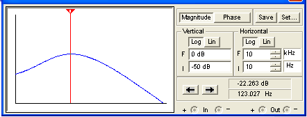
(The vertical scale is -50dB to 0dB.) Here we see that under real circuit conditions the attenuation is less dramatic and shifted downward in frequency.
Translating Theory into a Practical Design Strategy
To convert our analysis into a practical design procedure we need to translate the equations that determine the frequency response based on parts values into equations that determine parts values based on the desired frequency response. We take that step and put the formulas to practical use here:
The James Tone Stack: Creating Your Own Design.