How to Plot Intermodulation Distortion Using LTspice
We usually describe the frequency spectrum of guitar amp distortion in terms of harmonics. A single-ended power amp, for example, creates mostly second-harmonic distortion. A Fender Champ takes an 82Hz low-E fundamental from the guitar and adds a 6V6-generated second harmonic at 164Hz. For a 123Hz B fundamental, the amp adds a 246Hz harmonic. The push-pull circuitry of a Fender Deluxe produces mainly third-harmonic distortion, so instead we get 246Hz added to E and 369Hz added to B. The dynamics of harmonic distortion can be easily determined using SPICE and a good large-signal tube model.1,2 This tutorial shows how to plot another type of distortion: intermodulation distortion (IMD), the creation of frequencies that are not multiples of the fundamental. IMD is musically significant for power chords, as will be seen.
A Single-Ended Power Amp Example
Since we are examining a general concept, not designing a guitar amplifier as a complete system,3 let's use a known example from a 6L6 data sheet.
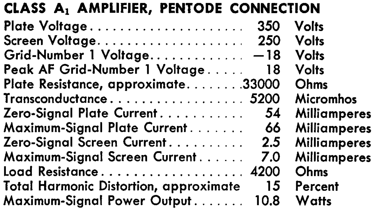
This example is convenient because the screen-to-cathode voltage is 250V, allowing us to use published 6L6 plate characteristics for a 250V screen.
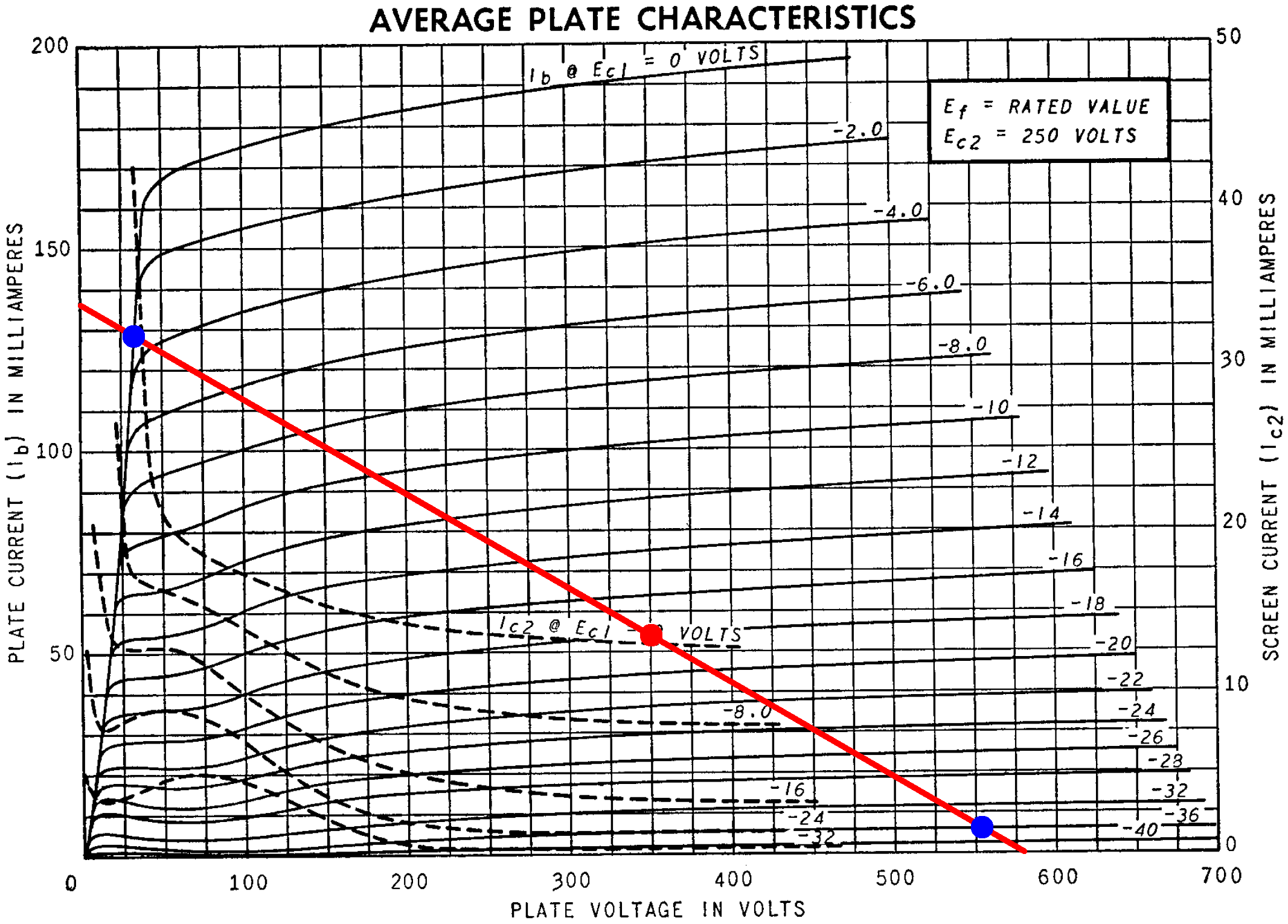
The DC operating point (red dot) is at a plate voltage of 350V, a plate current of 54mA, and a grid voltage of -18V. The red load line is for a 4.2kΩ output transformer primary impedance. Full power is achieved with an 18V peak signal at the grid, which causes the plate voltage and plate current to swing between the two blue dots. The grid-to-cathode voltages, plate-to-cathode voltages, and plate currents are
- VGK = 0V, VPK = 39V, IP = 139mA, and
- VGK = -36V, VPK = 580V, IP = 6mA.
These points, together with the DC operating point, can serve as references to test the vacuum tube model incorporated into our schematic.4

|
Guitar Amplifier Electronics: Fender Deluxe - from TV front to narrow panel to brownface to blackface Reverb |
6L6 Model
We will use an Adrian Immler large-signal 6L6 model, which does an excellent job at capturing the nuances of beam power tetrode performance. An LTspice DC operating point simulation shows that the Immler model and the upper left blue point are in complete agreement: the plate current is 139mA for the specified electrode voltages.
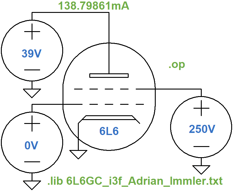
Here are the plate current values for the DC operating point and the lower right extreme of swing.
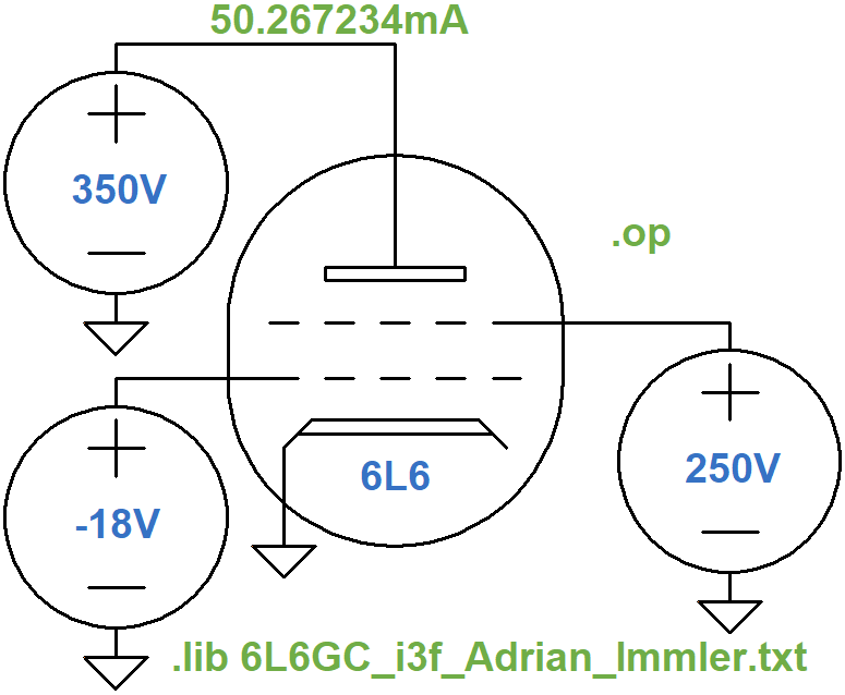
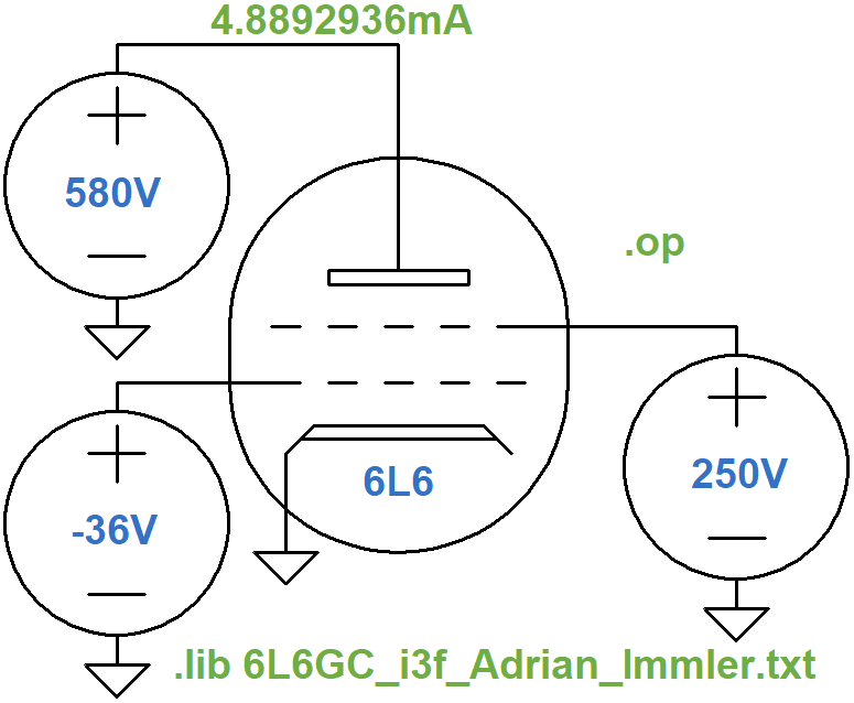
The model's plate current at the DC operating point and the lower-right blue point are within 4mA and 1mA, respectively, which is quite good.

|
Guitar Amplifier Electronics: Basic Theory - master the basics of preamp, power amp, and power supply design. |
Output Transformer Model
We need a single-ended output transformer with a primary impedance of 4.2kΩ and a secondary impedance of, say, 8Ω. The inductance ratio is equal to the impedance ratio,5 so if we arbitrarily set the primary inductance to 10H, the secondary inductance is
(10H)(8Ω / 4.2kΩ) = 19mH
To check this, let's set up a quick transient simulation for the transformer in isolation.
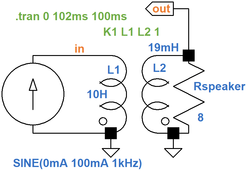
The K1 statement couples
the two inductors with an ideal magnetic coupling value of 1.
The current source has a sine function with a DC offset of 0mA, an amplitude of
100mA, and a frequency of 1kHz.
The .tran SPICE directive allows the simulation run for 100 milliseconds,
so that transients can die out,
and then records 2 milliseconds of data,
enough to plot two cycles of a 1kHz sine wave.
Here is the voltage across the 8Ω speaker and the current through it.
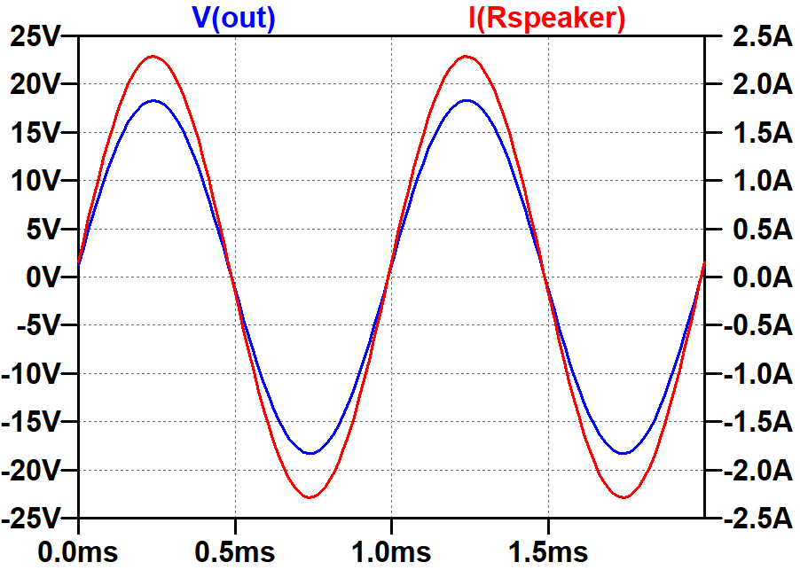
By holding down the control button and clicking on the plot labels V(out) and I(Rspeaker), we see the RMS voltage across the speaker and the RMS current through it.
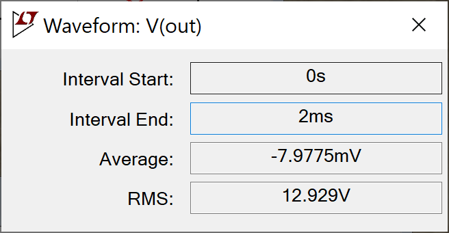
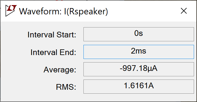
According to Ohm's Law, their ratio represents an impedance of
12.929V / 1.6161A = 8Ω
An impedance of only 8Ω represents a low-voltage, high-current environment, the kind that requires beefy copper speaker wires. Conditions in the primary are different: vacuum tubes operate in a high-voltage, low-current environment in which light-gauge wire is sufficient. Here is a plot of the voltage across the primary and the current through it.
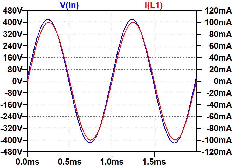
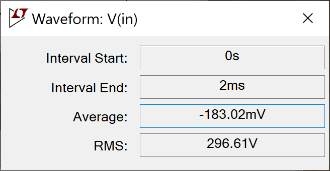
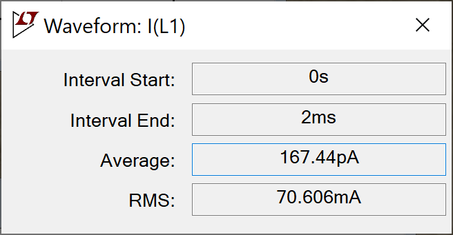
As expected, the primary impedance based on RMS values is
296.61V / 70.606mA = 4.2kΩ

|
Fundamentals of Guitar Amplifier System Design - design your amp using a structured, professional methodology. |
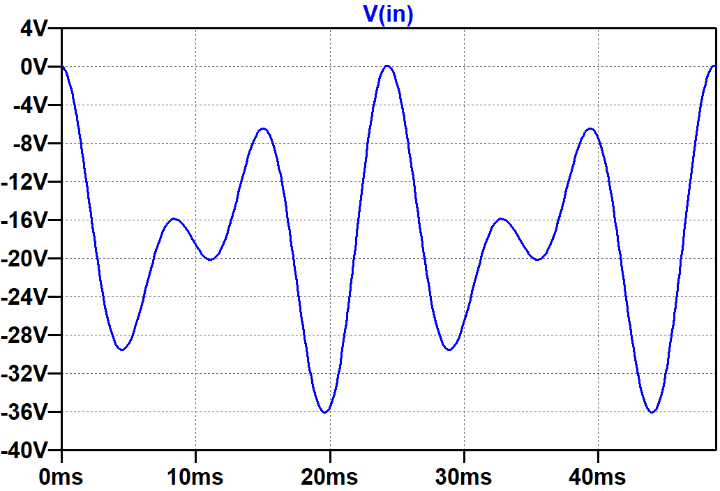
A Simple Mixer
Let's mix two input sinewaves: 82Hz (low E) and 123Hz (the B above low E). The difference between the two frequencies is 41Hz, which has a period of
1 / 41Hz = 24.39ms
The mixture therefore creates a wobbly waveform that repeats itself every 24.39 milliseconds. If we record data for double this time period, 48.78ms, then we get a snapshot of two cycles.
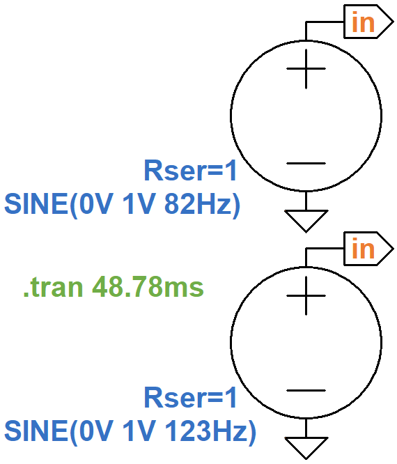
The voltage sources connected to node in have series resistances of 1Ω.
Each creates a Thevenin equivalent circuit 6
with an ideal voltage source and a 1Ω output impedance.
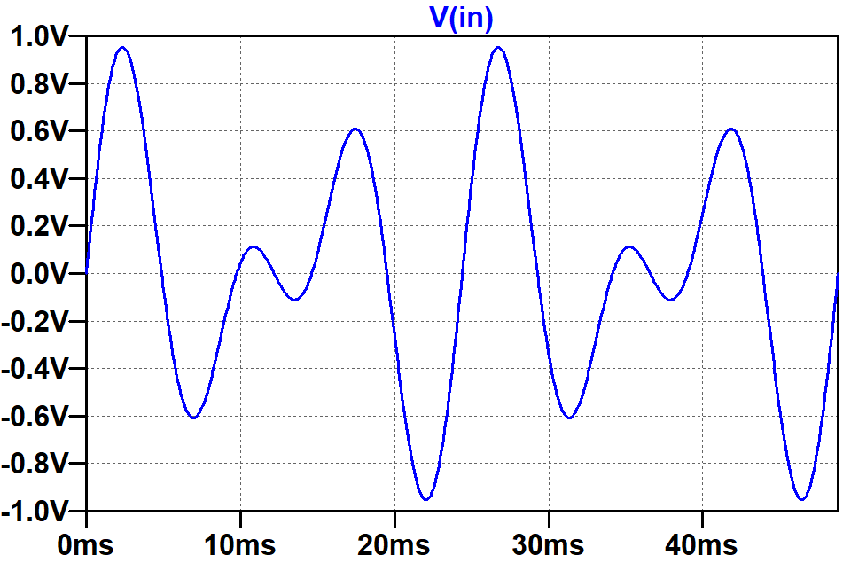
Here is the resulting voltage at node in.
|
Guitar Amplifier Electronics: Circuit Simulation - know your design works by measuring performance at every point in the amplifier. |
The IMD Simulation
We now have the three main components for simulating intermodulation distortion in the power amp:
- a large-signal vacuum tube model,
- an output transformer model, and
- a mixer to create the input signal.
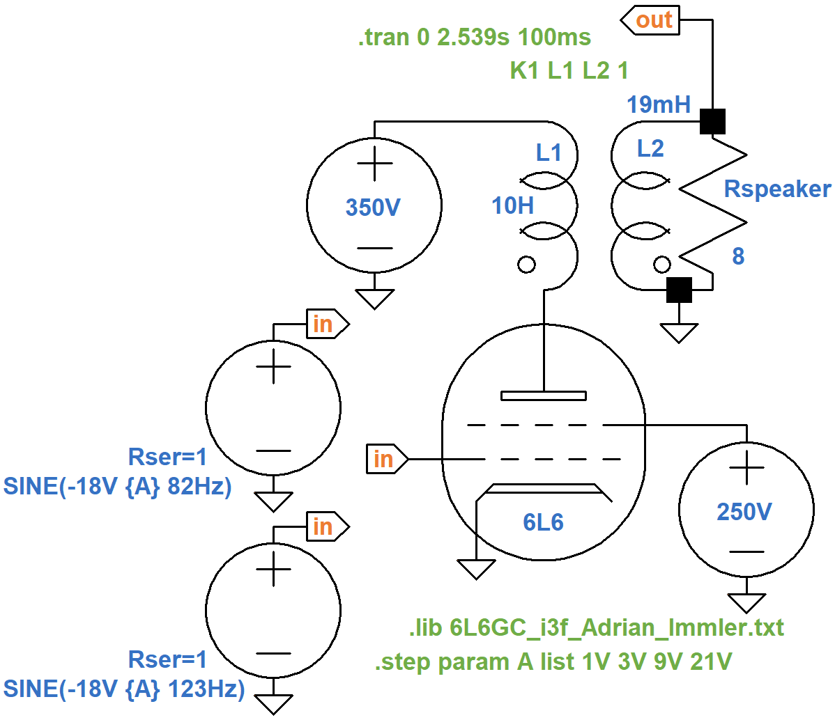
This schematic puts them all together.
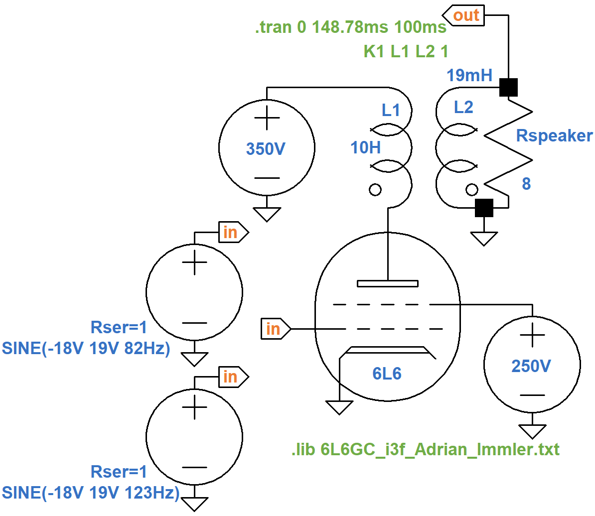
The .tran SPICE directive throws away the first 100 milliseconds
of data to allow transients to subside.
For the two input voltage sources,
the DC offset is set to -18V to set the DC grid bias.
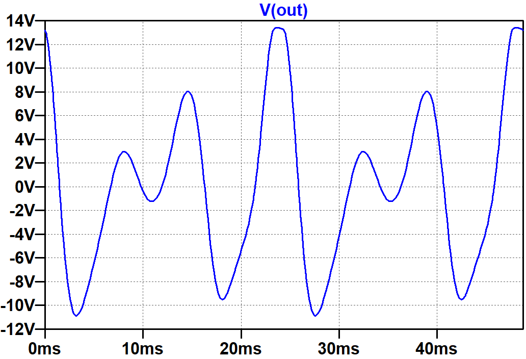
The amplitude of each source is set to 19V, which creates a maximum signal swing of 18V at the grid.
The speaker output is clearly distorted at the extremes of swing.
If a circuit is perfectly linear, it can change a signal's amplitude and phase but it cannot create frequencies that are not present in the input. If 82Hz and 123Hz are the only frequencies in the input, they are the only frequencies in the output. Nonlinear distortion adds new frequencies. To identify them we need to shift our perspective. Instead of displaying signal level versus time, let's display signal level versus frequency.
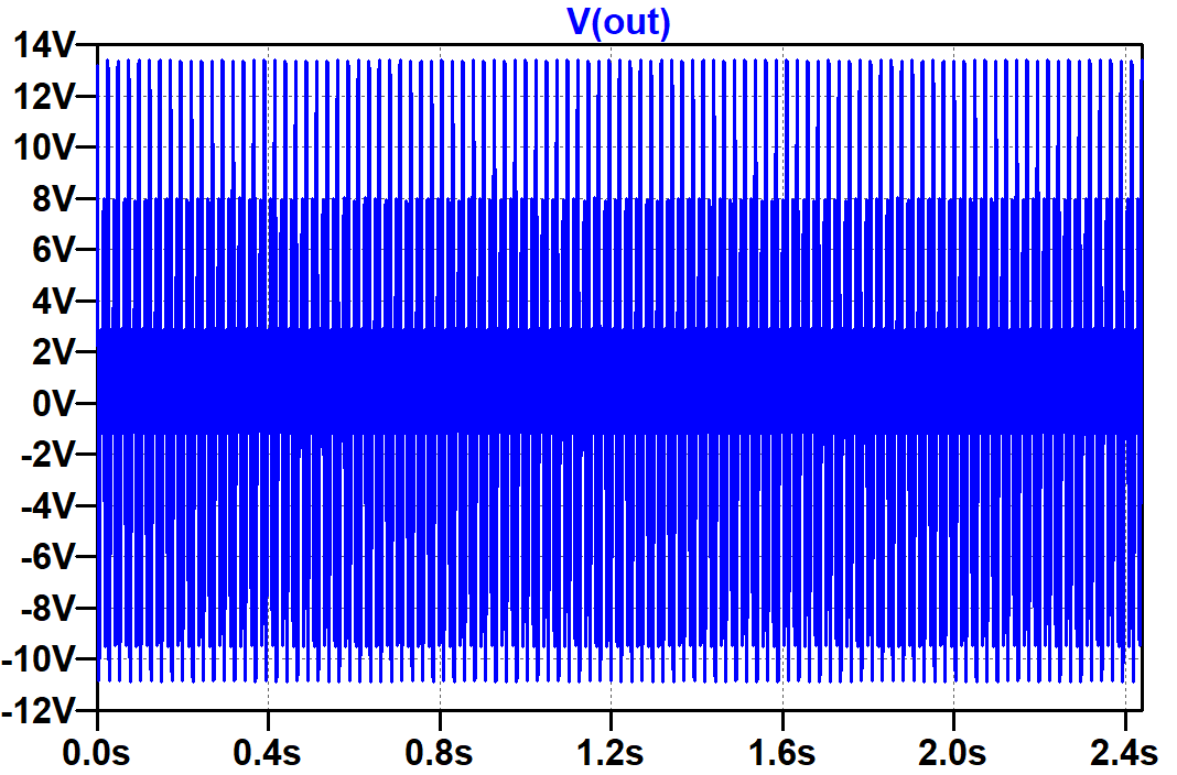
To get a big reservoir of time-domain data, let's extend the simulation time:
.tran 2.539s 100ms
The stop time is set to 2.539 seconds and the time to start recording data is at 100 milliseconds, so 2.439 seconds of data is recorded, enough for 100 periods of the input. For our time-domain plot, signal amplitude versus time for this many periods looks like a solid blob, which is not very informative.
If we right click on the plot window and then select
View > FFT
this window appears.
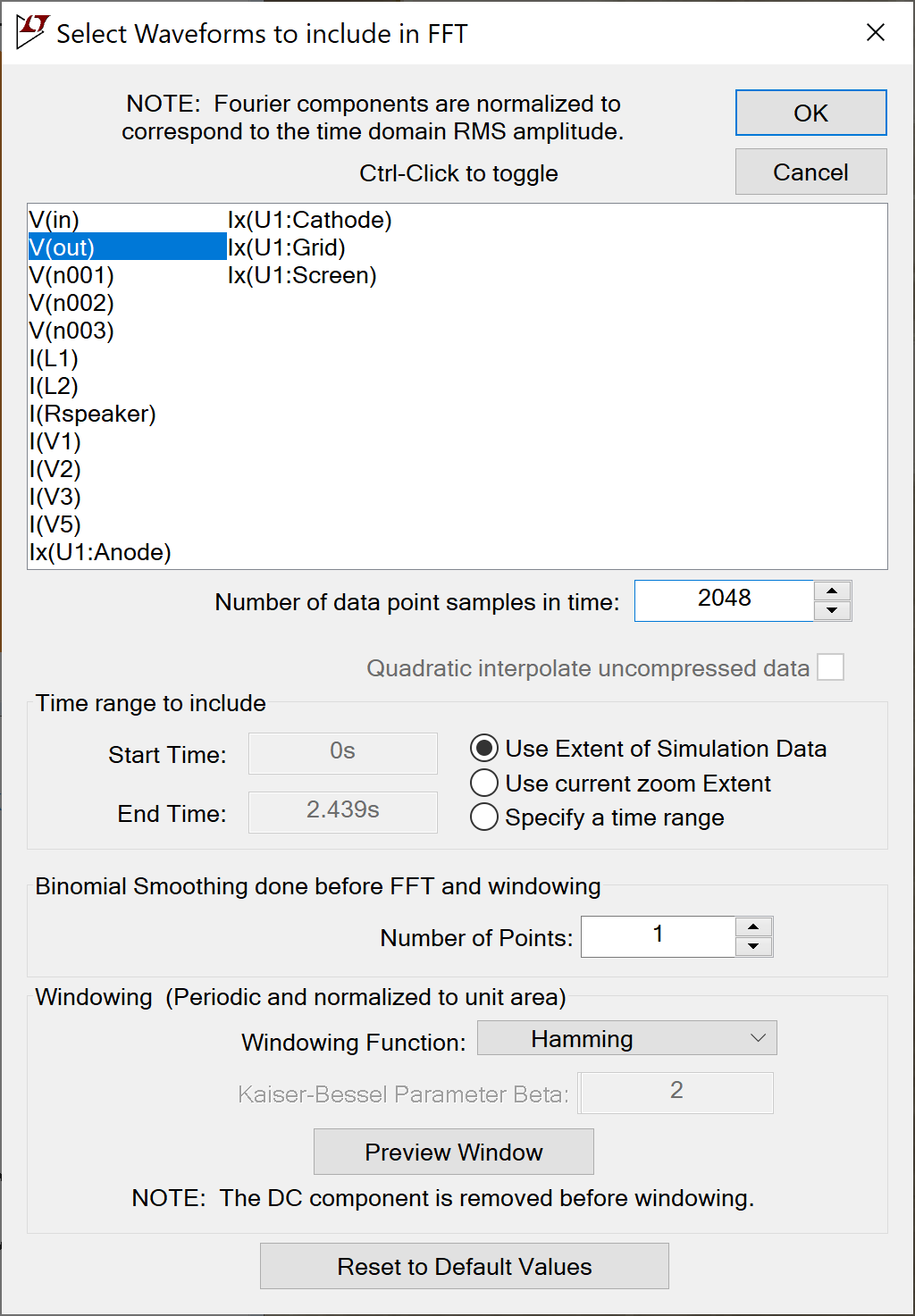
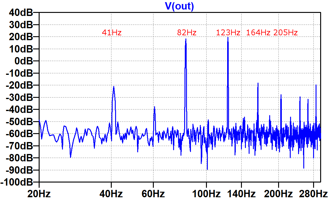
Engineers, mathematicians, and physicists take a keen interest in the number of data point samples, the number of points used for binomial smoothing, and the type of windowing function. For our purposes, 2048 data points (a power of 2), 1 smoothing point (i.e. no smoothing), and a Hamming (raised cosine) window do the job. Here is the resulting FFT plot.
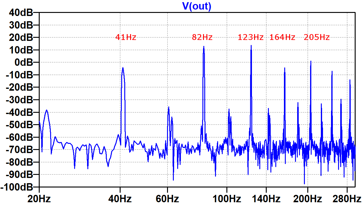
(The frequency labels in red have been manually added to the image.) The first spike represents the difference between the frequencies at the input:
123Hz - 82Hz = 41Hz
This is one component of intermodulation distortion (IMD), the amplitude modulation of the two input signals caused by the nonlinear circuit. The mathematics of the 41Hz difference in frequency has musical consequences. When the input contains the root and the fifth of a power chord, the fifth has a fundamental that is 1.5 times the frequency of the root fundamental. The difference is a new frequency that is 0.5 times the frequency of the fundamental, i.e. one octave lower. By adding this tone, the amp thickens the guitar signal.
The next two spikes are the input signal frequencies, which dominate the output despite the additional frequencies added to the mix. This is a good thing, because the human ear still perceives the result to be a low E and the B above it. The spike at 164Hz is the second harmonic of 82Hz. Harmonic distortion for a single-ended power amp is primarily the second harmonic until overdrive creates symmetrical clipping to bring up the third. The next spike is another IMD component, the sum of the input frequencies:
82Hz + 123Hz = 205Hz
The next spike (unlabeled) is the second harmonic for the 123Hz input signal: 246Hz.
To see how distortion develops as the signal level increases, let's step the input signal amplitudes through four values: 1V, 3V, 9V, and 21V. Full power is achieved with 19V, so the first three levels create less than full power and the last puts the power amp into overdrive.
Let's zoom in on the relationship between the 123Hz input frequency, the 164Hz harmonic, and the 205Hz IMD component.
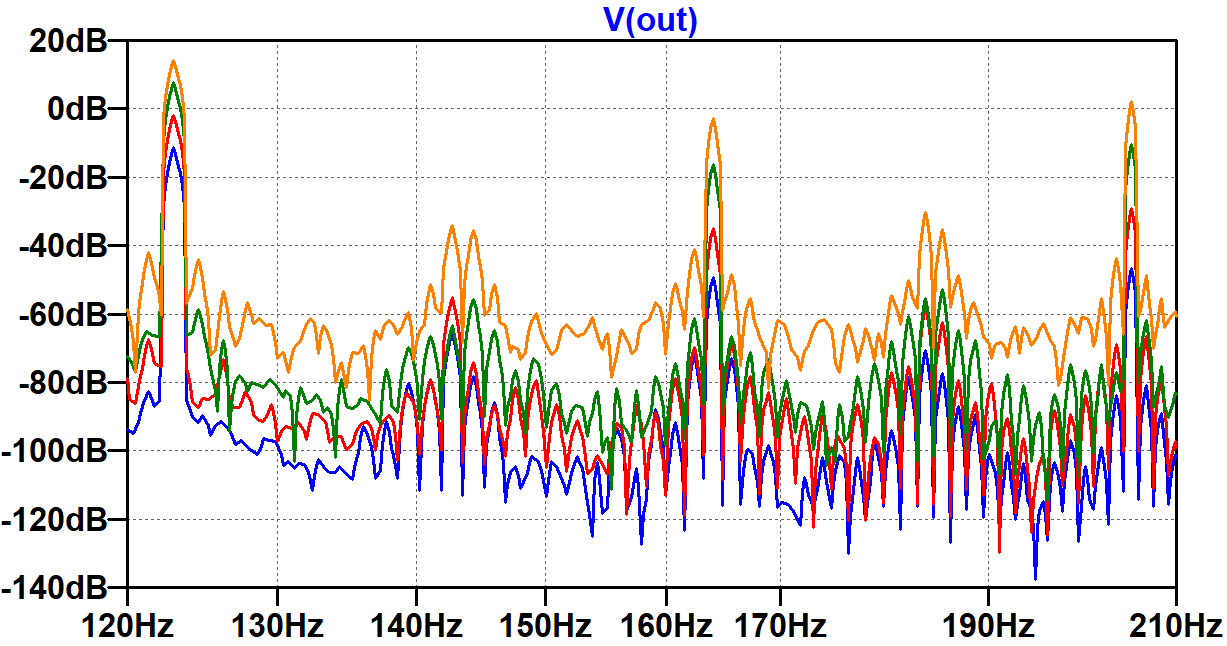
As the signal level approaches full power, the harmonic and IMD levels increase at a faster rate than the input frequency. To a guitar player this makes sense: as the guitar is cranked up, the overall signal level increases, but distortion frequencies increase at a faster rate.
A Push-Pull Power Amp Example
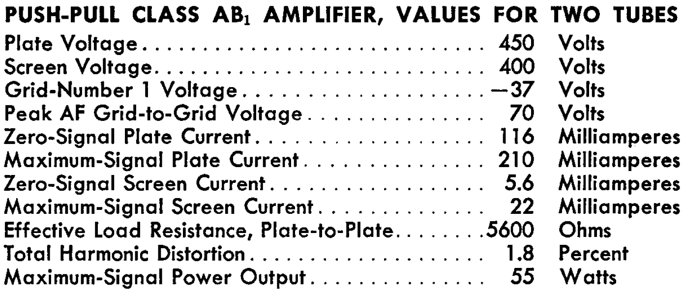
For a push-pull power amp, let's use another example from the data sheet.
Here is a test circuit to validate the tube model for the higher electrode voltages.
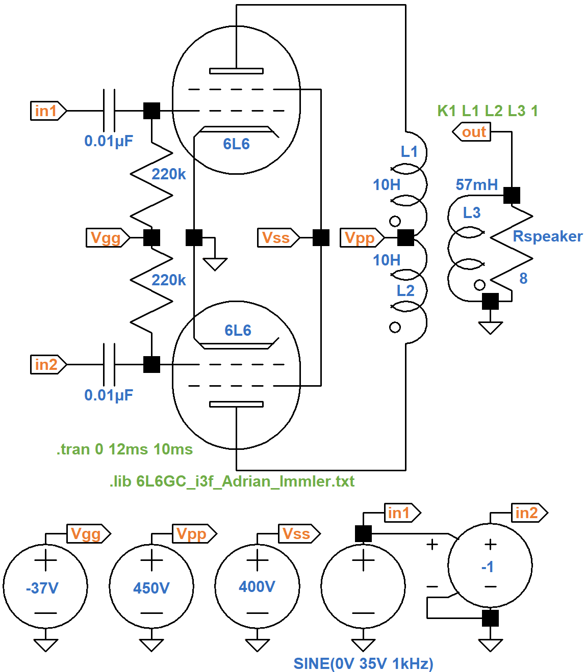
The output transformer primary impedance is 5.6kΩ plate-to-plate. Let's arbitrarily set the inductance of each half of the primary to a value of 10H. Normally the total inductance of two inductors in series is equal to the sum of their individual inductances. If L1 and L2 were chokes, for example, the total inductance would be 20H. Our inductors are magnetically coupled, however, so we use 40H for the purposes of determining the secondary inductance needed to drive an 8Ω speaker:
(8Ω / 5.6kΩ)(40H) = 57mH
The data sheet example specifies a "peak AF grid-to-grid voltage" of
70V to drive the power amp to 55 watts.
To set this up, we have a voltage source driving node in1
with a 35V peak, 1kHz sine wave.
It drives a voltage-controlled voltage source with a coefficient of -1
to create an identical signal of opposite phase at node in2.
This mimics the performance of a phase inverter.
The transient simulation is set to run for 10 milliseconds and then
collect data for 2 milliseconds to capture 2 cycles of the 1kHz signal.
Here is the voltage across the speaker (blue),
the current through it (red),
and the instantaneous power level (green).
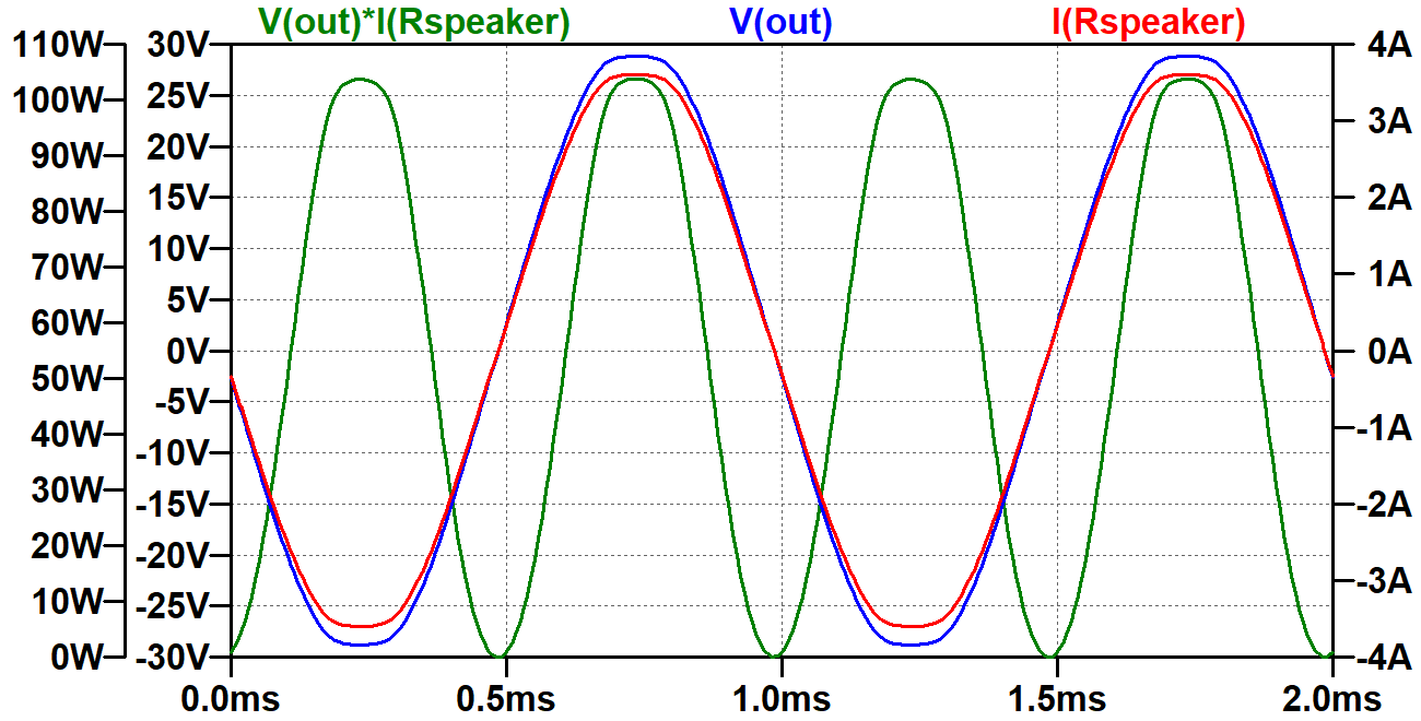
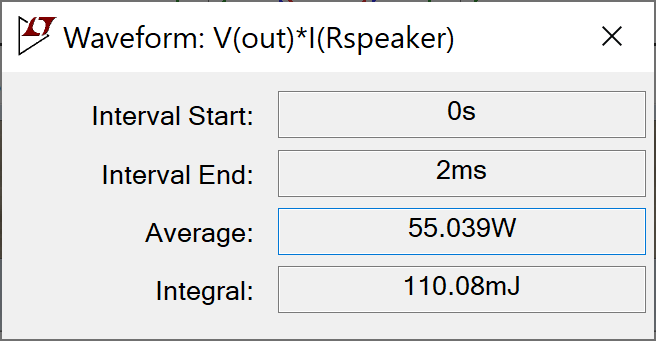
The RMS output power is an exact match to the data sheet specification: 55W.
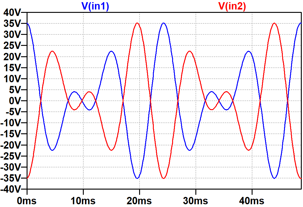
Like we did for the single-ended power amp, we set up a mixer for 82Hz and 123Hz. When the individual amplitudes are 36.9V, the mix swings plus or minus 35V.
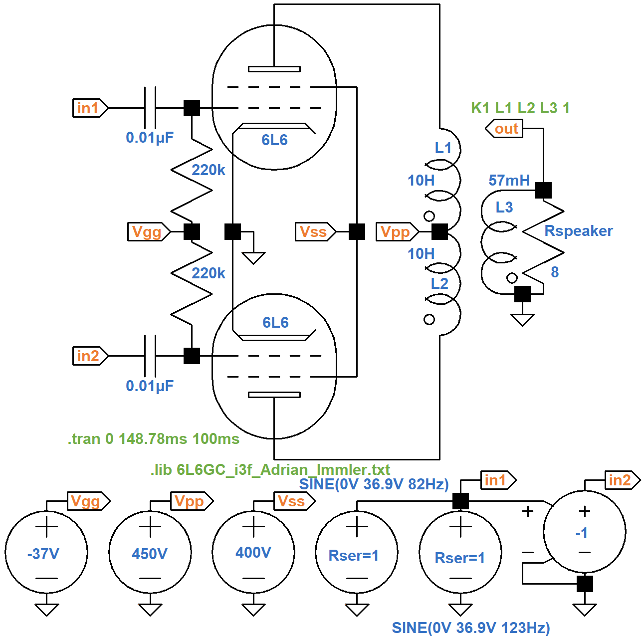
The inputs are identical but of opposite phase.
We set up to record 100 periods of the signal:
.tran 0 2.539s 100ms
Here are the results when we view the FFT of the speaker voltage.
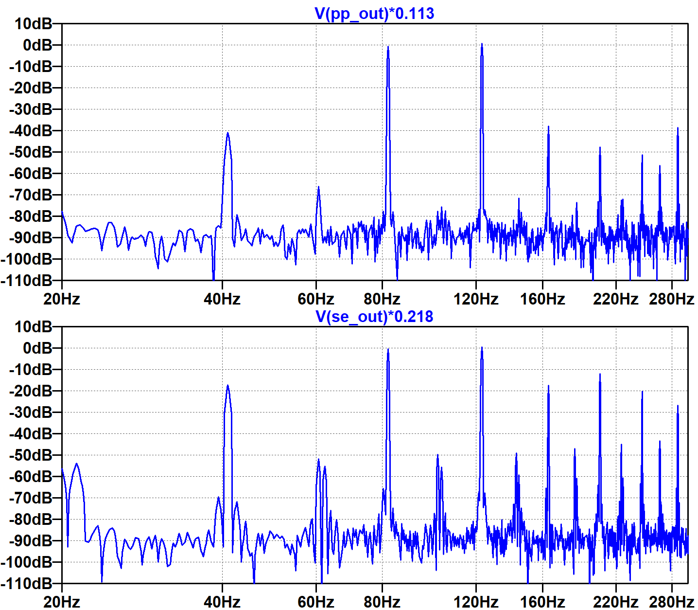
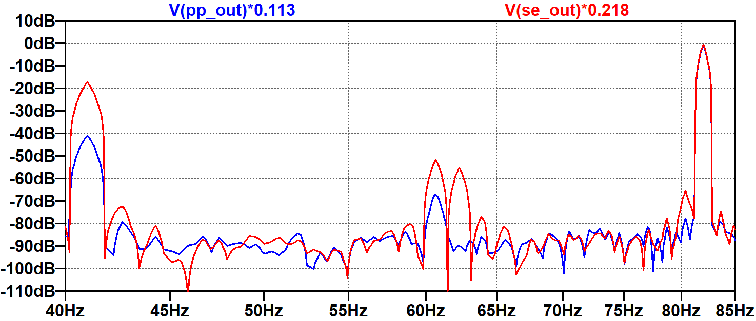
For direct comparison, here are the push-pull and single-ended results, both normalized to display dB relative to the input signals.
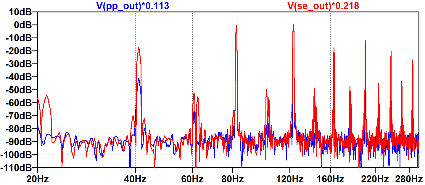
Here we include both traces in the same plot.
Here we zoom in on the 41Hz IMD component and the 82Hz input.
Finally, we zoom in on the 123Hz input, 164Hz harmonic, and 205Hz IMD component.
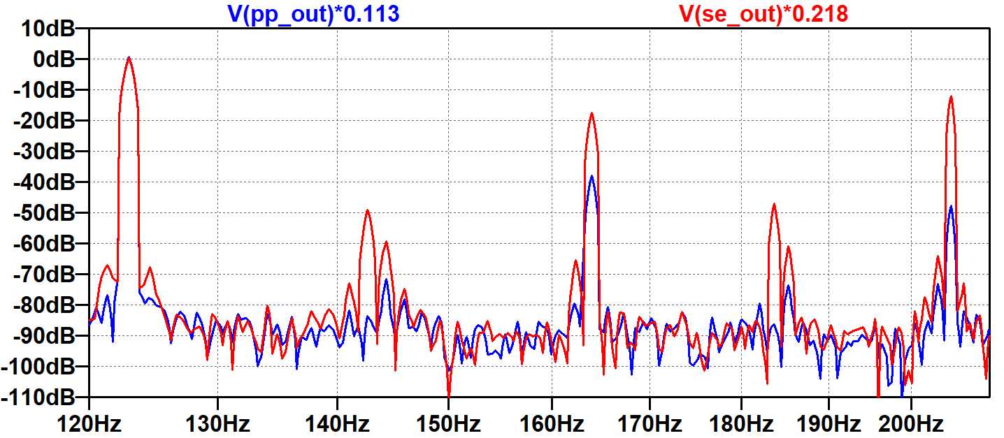
These plots demonstrate that the amplitude of each IMD component depends on the power amp's specific nonlinear behavior. It also depends on the amplitudes and phases of the two or more input sine waves being distorted. We have tested only one combination. It is therefore difficult to make broad generalizations based on these plots. We can only surmise that, under our specific test conditions, the single-ended design creates significantly more harmonic and intermodulation distortion. The thin sound of two sine waves becomes substantially thicker as a result.
References
1Richard Kuehnel, Guitar Amplifier Electronics: Basic-Theory, (Seattle: Amp Books, 2018), pp. 173-177.
2Richard Kuehnel, Guitar Amplifier Electronics: Circuit Simulation, (Seattle: Amp Books, 2019), pp. 135-145, 187-191.
3Richard Kuehnel, Fundamentals of Guitar Ampliier System Design, (Seattle: Amp Books, 2019).
4Richard Kuehnel, Guitar Amplifier Electronics: Circuit Simulation, (Seattle: Amp Books, 2019), pp. 86-99.
5Richard Kuehnel, Guitar Amplifier Electronics: Basic-Theory, (Seattle: Amp Books, 2018), pp. 27-28.
6Richard Kuehnel, Guitar Amplifier Electronics: Basic-Theory, (Seattle: Amp Books, 2018), p. 68.