Digital Modeling of Guitar Amplifier Preamp Distortion
Gone are the days of applying a single, overly simplistic sigmoid function to a sample sequence to digitally model the distortion of an entire guitar amplifier. Modern models include accurate emulation of both preamp and power amp distortion based on actual circuits. Consider, for example, this preamp stage.
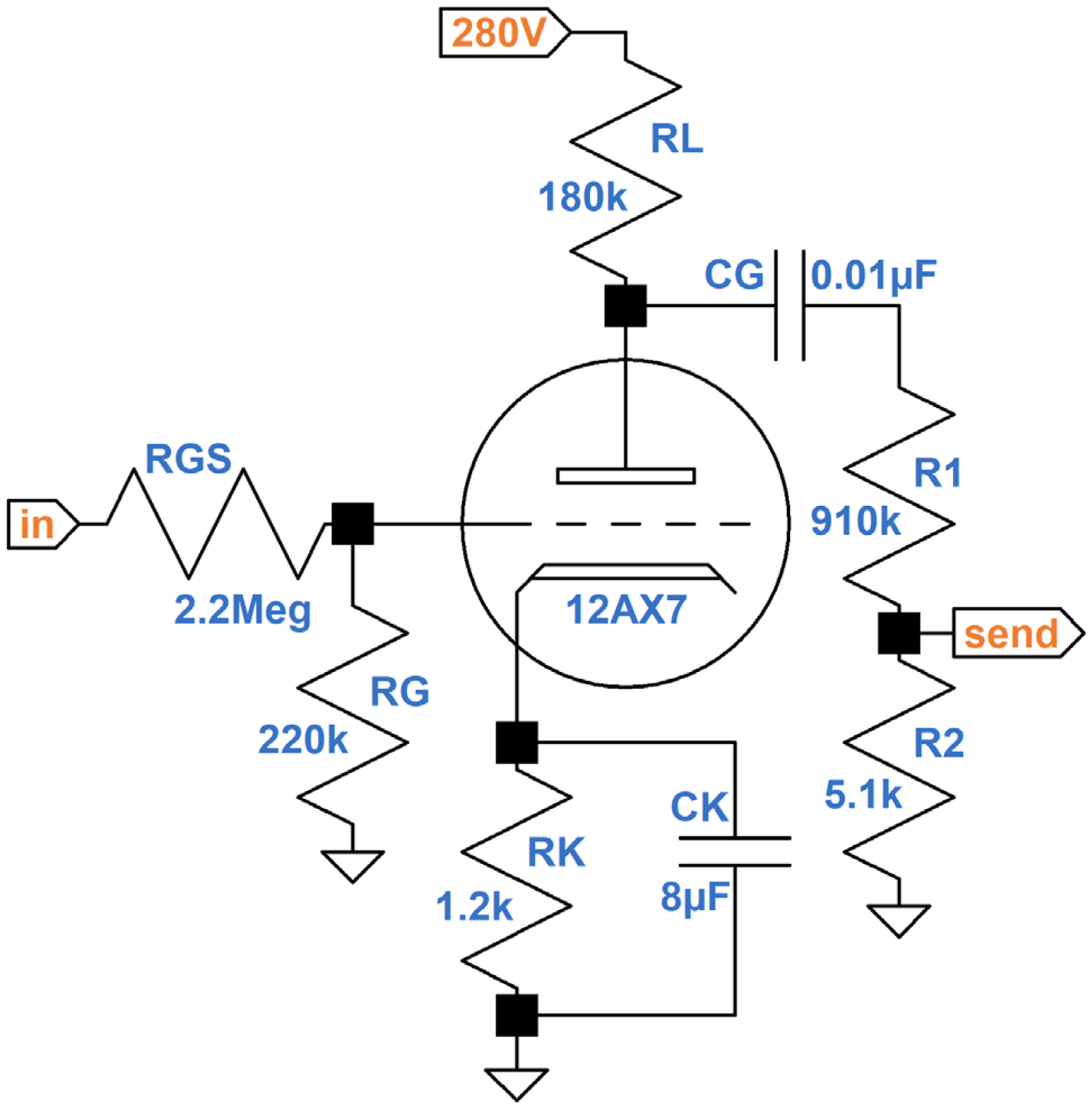
This is the final stage of a preamp designed to drive an effects loop and is the first preamp stage to break into distortion. The design is similar to the preamp distortion stage in the Mesa/Boogie Mk I.
The cathode resistor is fully bypassed to prevent negative feedback from reducing the triode circuit's lush nonlinear behavior. R1 and R2 form a voltage divider to reduce a maximum plate voltage swing of about 100V peak to a maximum effects send swing of about half a volt peak.
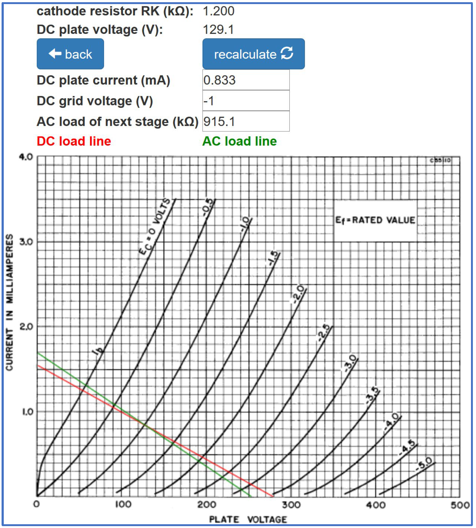
According to the 12AX7 Calculator, the grid is biased at a very warm -1V.
As the input signal level increases, positive grid voltage swings are compressed by the effects of grid current on the upstream resistor network. Negative swings of the input signal run free. The severe asymmetry produces bucketloads of 2nd-harmonic distortion that plateaus early and lasts until negative grid voltage swings reach approximately -3V. At that point, peak-to-peak plate voltage swing has almost reached its limits.
When negative grid voltage swings exceed -3.5V, positive plate voltage swings transition from mild compression to sharp clipping. The output waveform becomes more symmetrical and 3rd-harmonic distortion begins to dominate. Beyond that point the output signal is at its maximum - it cannot respond to further increases in input signal amplitude.

|
Guitar Amplifier Electronics: Fender Deluxe - from TV front to narrow panel to brownface to blackface Reverb |
Traditional Waveshapers
Guitar amp nonlinear behavior has traditionally been modeled by a waveshaper, which describes the output as a function of the input. Here, for example, is a waveshaper included in a Line 6 patent.2
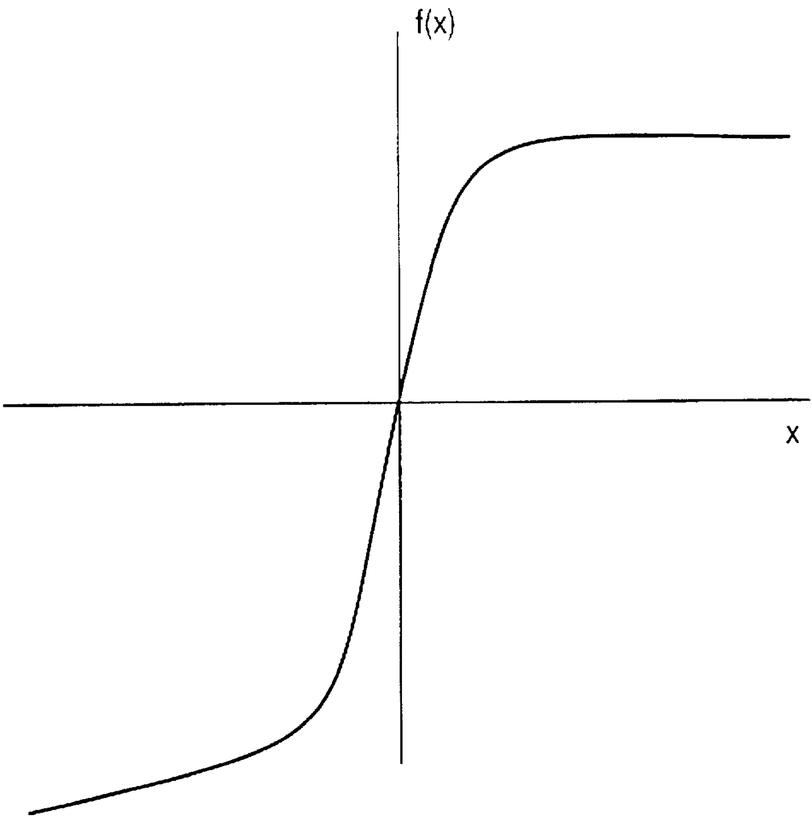
For a linear circuit the transfer function is a straight line. The Line 6 waveshaper shows compression at the extremes of positive and negative input swings. It also depicts asymmetric distortion, because the curve for positive voltage swings is not the mirror image of the curve for negative swings.

|
Guitar Amplifier Electronics: Basic Theory - master the basics of preamp, power amp, and power supply design. |
A More Accurate Model
"Most products now use a single dynamic waveshaper to simulate the entire nonlinear response of the amplifier. The Axe-Fx II uses a highly sophisticated approach that involves multiple triode simulators and a dedicated power amp simulator. It is our firm belief that multiple distortion stages can only be accurately simulated using multiple digital stages of distortion, especially separate preamp and power amp simulations as the distortion contributed by each is unique and the best tones are achieved through a combination of preamp and power amp distortion." 3 - Fractal Audio Systems
The model for our preamp stage will be divided into two components:
- a waveshaper-like transfer function that captures nonlinear behavior and
- a high-pass filter that captures the low-frequency behavior of coupling capacitor CG.
Here are the results of a SPICE simulation1 for a quarter cycle of a 1kHz sine wave input with
an amplitude of 32V,
which is sufficient to put the stage well into overdrive.
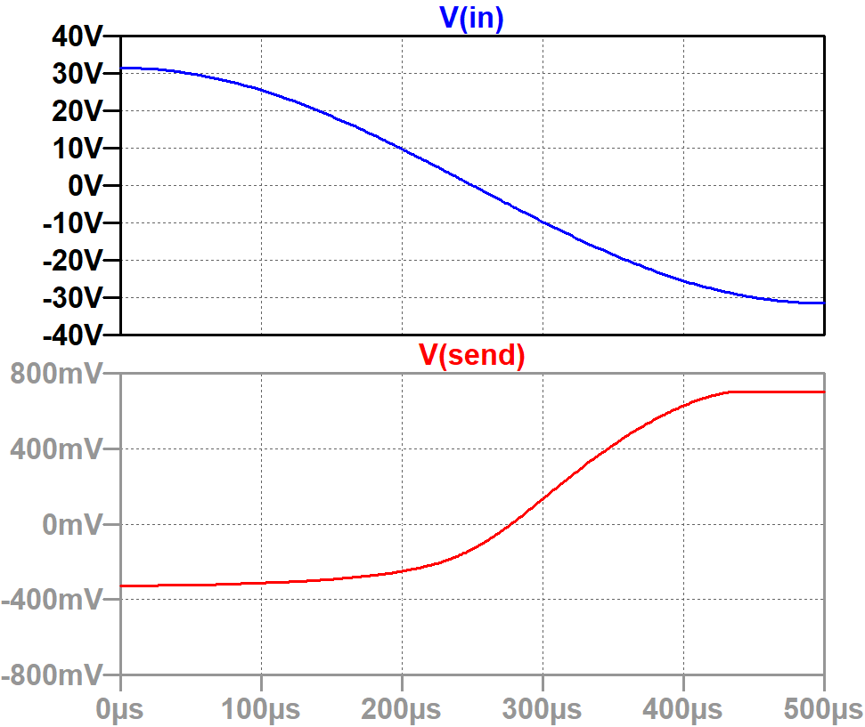
For the simulation, the coupling capacitor value is set to 100μF to eliminate its low-frequency effects. Post-distortion behavior will be emulated separately via a high-pass digital filter.
|
Fundamentals of Guitar Amplifier System Design - design your amp using a structured, professional methodology. |
Cubic Spline Interpolation of the Transfer Function
To normalize and reverse the phase of the input, we can multiply its values by -1/32.
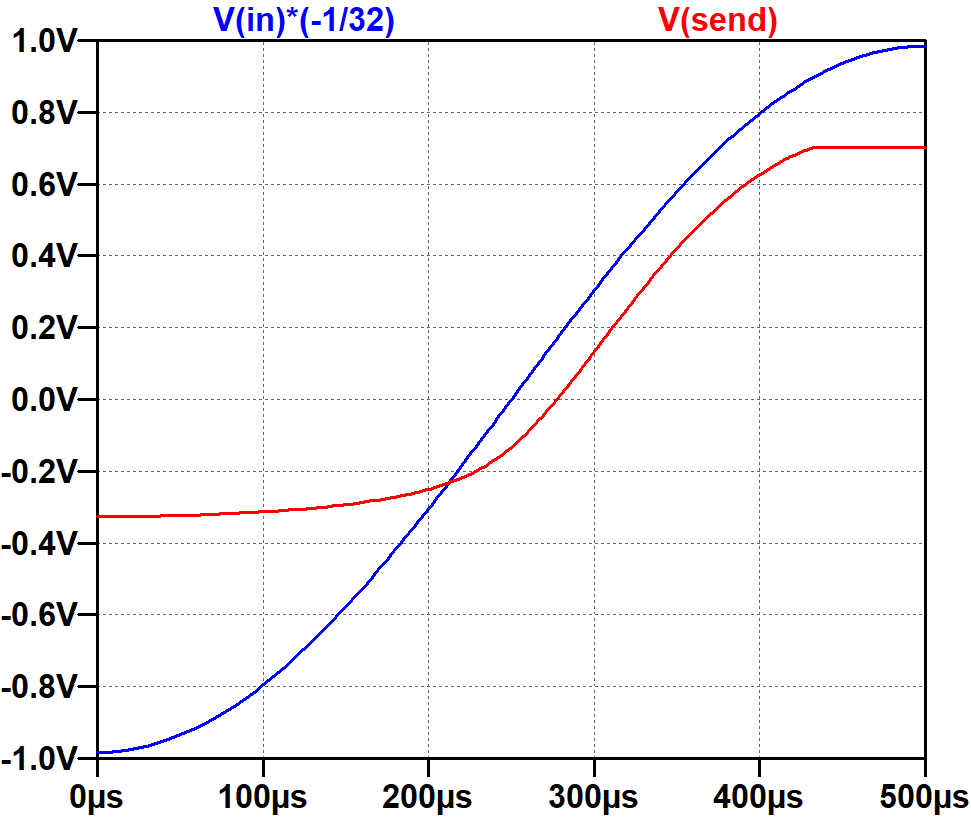
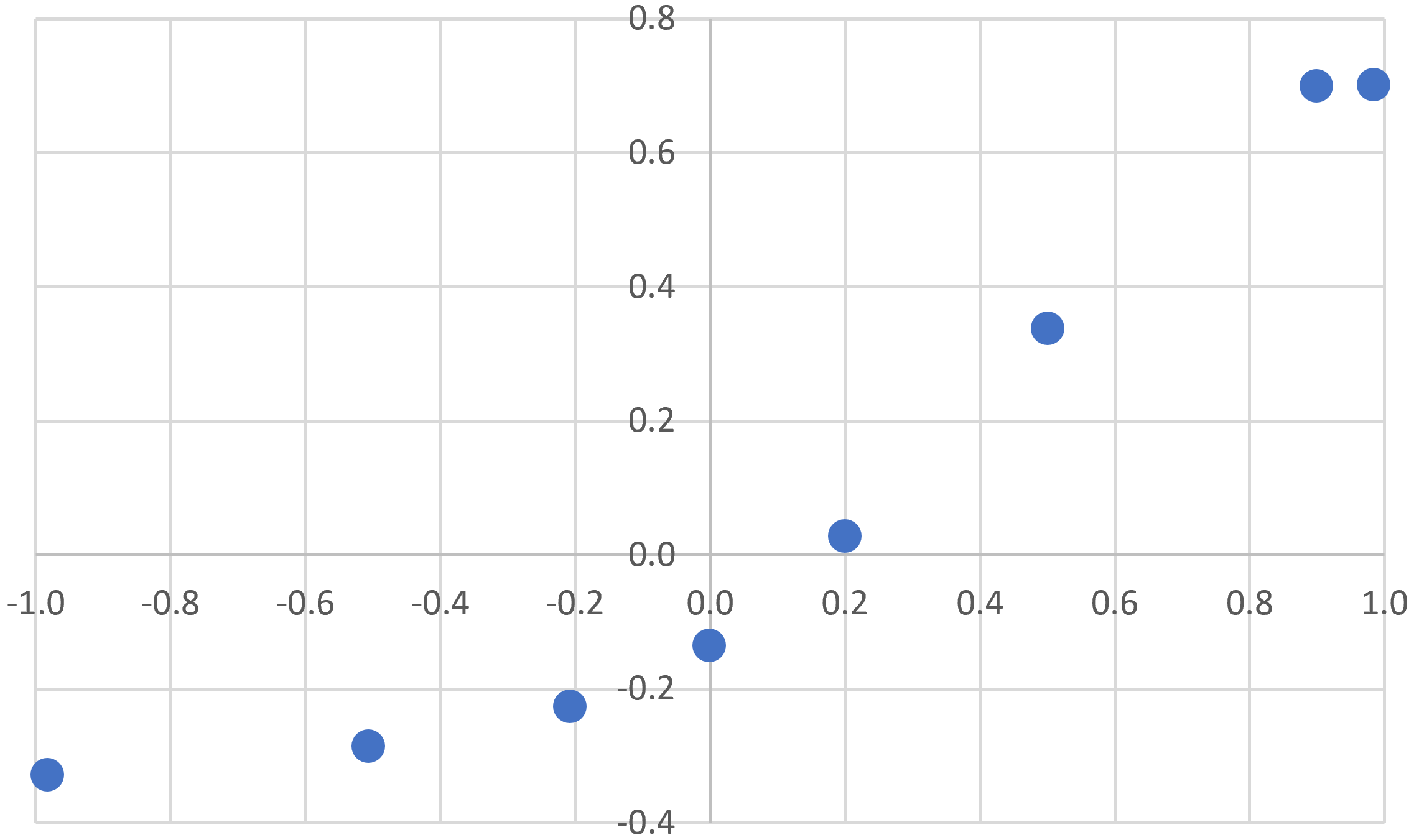
Next we can export the simulation results to a spreadsheet, where time is eliminated and the output is displayed as a function of the input.
This represents the transfer function that we want to model. Let's pick some key points for fitting a mathematical curve to the data.
| x | f(x) |
| -0.98338 | -0.32623 |
| -0.50698 | -0.28419 |
| -0.20759 | -0.22581 |
| -0.00212 | -0.13455 |
| 0.20041 | 0.02867 |
| 0.50062 | 0.33908 |
| 0.89961 | 0.70177 |
| 0.98453 | 0.70220 |
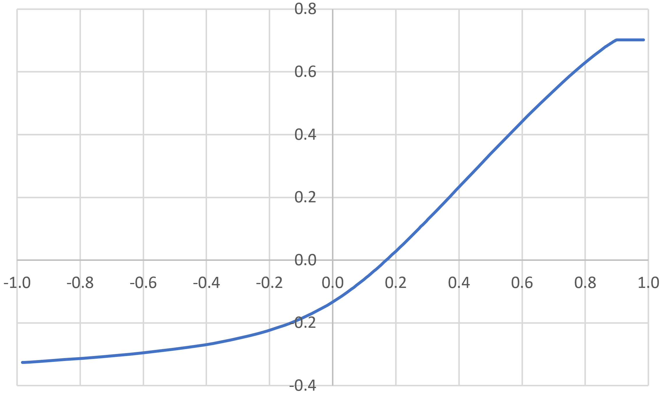
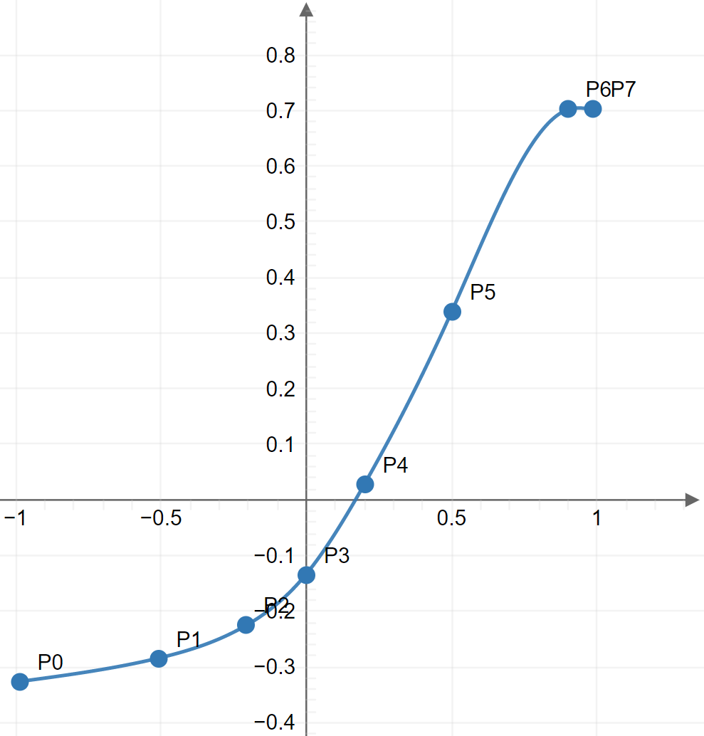
We can use an online tool for cubic spline interpolation4 to fit a curve to all but the last point. If we include the last point, then interpolation removes the sharp transition to cutoff, as shown here.
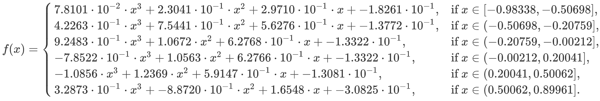
With the final point eliminated, we can manually limit the output to a value of 0.7 when the input exceeds 0.9, thereby replicating the sharp cutoff beyond point P6.
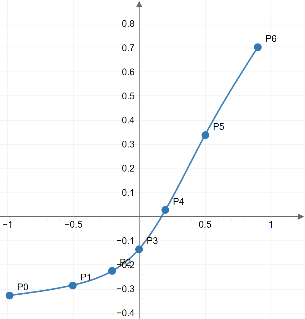
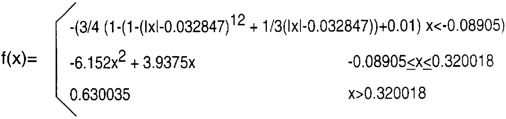
Here is the resulting mathematical model for the transfer function, to which we can add that f(x) = -0.32623 when x is less than -0.98338 and f(x) = 0.70177 when x is greater than 0.89961.
|
Guitar Amplifier Electronics: Circuit Simulation - know your design works by measuring performance at every point in the amplifier. |
A Digital High-Pass Filter to Emulate the Coupling Capacitor
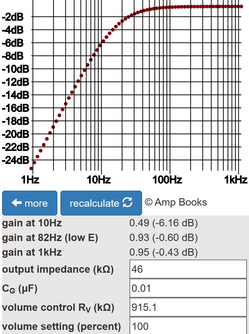
According to the Preamp Gain and Output Impedance Calculator, the output impedance driving the coupling capacitor and effects send voltage divider is 46kΩ. (This assumes linear conditions but without significant consequences.) The stage has an AC load of 915.1kΩ created by R1 and R2 in series.
According to the Coupling Capacitor Calculator, there is 0.6dB attenuation at 82Hz, the lowest note on a guitar with standard tuning.
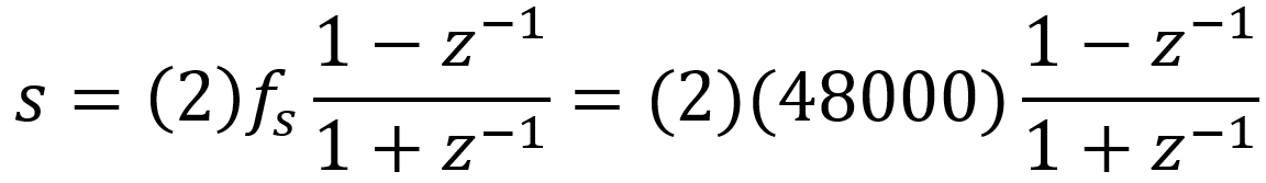
The response of the analog circuit in terms of the Laplace variable s is
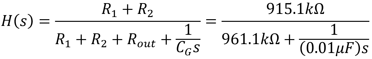
The relationship between the coefficients of the digital filter and the coefficients for the analog filter depends on the sample rate fs. Let's assume a 48kHz sample rate. Using a bilinear transform, we substitute this expression for the analog variable s:
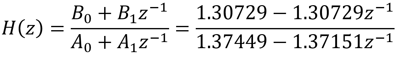
Here are are the resulting coefficients for the digital filter.
The expression z-1 represents a delay by one sample. The frequency response for the digital filter, as a function of z, is the output divided by the input:
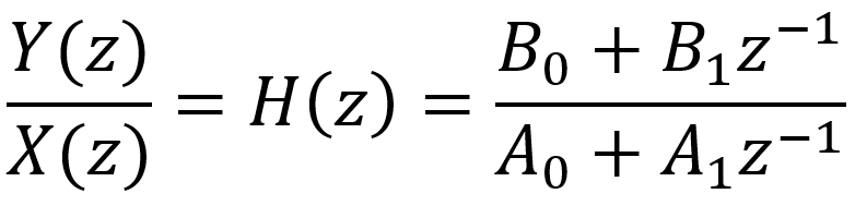
The relationship between the input and output is therefore

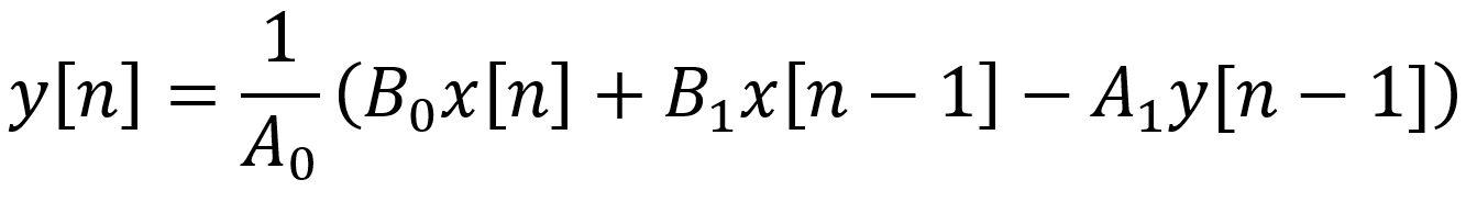
Since each z-1 represents a delay of 1 sample, in the time domain we get

This is the formula we use to actually code the digital filter in C++ or the Rust programming language. Specifically, the current output sample is
Here is the digital filter's response plotted by GNU Octave.
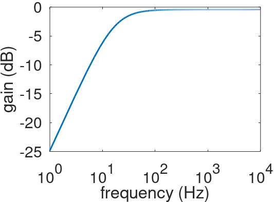
At a sample rate of 48kHz, there is no discernable difference between this response and the response of the analog circuit shown earlier.
Finalizing the results
Our model combines a nonlinear transfer function and a high-pass filter. Before it can be implemented, one task remains: oversampling, as shown here in a Line 6 patent.
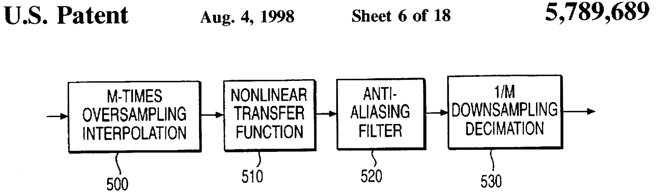
Oversampling is required because the nonlinear transfer function creates new harmonic frequencies substantially higher than the frequencies contained in the input. These frequencies can alias into lower frequencies, creating discernable artifacts known as foldover noise that are not present at the output of the analog circuit.
The Line 6 patent, for example, uses a sample rate of 31.2kHz and 8-times oversampling to create an effective sample rate of 249.6kHz upstream of the nonlinear transfer function. The seven new samples between each pair of existing samples are linearly interpolated, so a straight line is essentially drawn between every two existing samples and 7 new sample points are selected along it.
The transfer function is applied to the oversampled signal, which then passes through a low-pass anti-aliasing filter to eliminate foldover noise. The signal is then decimated back to the original sample rate by retaining only 1 out of every 8 samples in the output.
If oversampling is used upstream of our high-pass filter, then the coefficients A0, A1, B0, and B1 need to be determined based on the faster sample rate.
References
1Richard Kuehnel, Guitar Amplifier Electronics: Circuit Simulation, (Seattle: Amp Books, 2019).
2U.S. Patent 5,789,689.
3Fractal Audio Systems, Multipoint Iterative Matching and Impedance Correction Technology (MIMICTM), April 2013, p. 5.
4Timo Denk, "Online Tools," Available at https://tools.timodenk.com/cubic-spline-interpolation (Retrieved February 23, 2020)